Probability – Complete Guide For Class 12 Math Chapter 13

Welcome to iPrep, your Learning Super App. Our learning resources for the chapter, Probability in Mathematics for Class 12th are designed to ensure you grasp this concept with clarity and perfection. Whether you’re studying for an upcoming exam or strengthening your concepts, our engaging animated videos, practice questions and notes offer you the best of integrated learning with interesting explanations and examples. 

The chapter Probability explores the mathematical framework for analyzing random events and predicting outcomes. It introduces students to important concepts such as conditional probability, Bayes’ theorem, and random variables. The chapter also covers the binomial distribution, the concept of independence, and the application of probability in various real-life scenarios. Understanding probability is essential for advanced studies in fields like statistics, economics, genetics, and machine learning, where it plays a critical role in decision-making, data analysis, and risk assessment.

Probability

In our daily lives, we often encounter situations where the outcome is uncertain. For instance:

• When we wake up and check the weather, we might see a statement like “There is a 60% chance of rain today.”
• While deciding what to eat for breakfast, we might consider the statement “Corn flakes might reduce cholesterol.”
• We may wonder, “What are the chances of getting a flat tire on the way to an important appointment?”

These situations are governed by the concept of probability, which helps us measure the likelihood of uncertain events. Thus the definition of probability can be 

Probability is the branch of mathematics devoted to the study of such events. 

Conditional Probability

Conditional probability answers the question: If two or more events arise from the same sample space, does the occurrence of one event affect the probability of the other? To explore this, consider an experiment involving the selection of a card from a deck of ten cards numbered 0 to 9. The sample space is:

S = {0,1,2,3,4,5,6,7,8,9}

Each outcome has a probability of 1/10. Let event A be “the number on the card is even,” and event B be “the number on the card is greater than 3.”

For event A:  

A = {0,2,4,6,8} 

P(A) =  P(0) + P(2) + P(4) + P(6) + P(8)

          = 1/10 + 1/10 + 1/10 + 1/10 + 1/10   = 5/10 = 1/2

For event B: 

B = {4,5,6,7,8,9} 

P(B) = P(4) + P(5) + P(6) + P(7) + P(8) + P(9)

         = 1/10 + 1/10 + 1/10 + 1/10 +1/10 + 1/10 ​ = 6/10 = 3/5

 The intersection of A and B (common elements) is: 

  A∩B = {4,6,8} 

P(A∩B) = P(4) + P(5) + P(6)    

                = 1/10 + 1/10 + 1/10 = 3/10 =    

Now, if we know that event B has occurred, the probability of A changes. The sample space for A becomes restricted to the outcomes favorable to B:

Sample points of A favorable to B: {4,6,8} 

P(A∣B)= 1/6 + 1/6 +1/6  = 3/6 = 1/2

Thus, the conditional probability of A given B is: P(A∣B) = P(A∩B) / P(B) 

                                         = 3/10 / 6/10 = 3/10 x 10/6 = ½

Based on the previous discussion, we define the conditional probability as follows: 

If E and F are two events associated with the same sample space of a random experiment, the conditional probability of the event E given that event F has occurred, i.e., P(E | F) is given by = P(E∩F) / P(F), provided P(F) ≠ 0 

​

Properties of Conditional Probability

Let us make some assumptions before starting to learn the properties of conditional probability. 

• Let us take S as a sample space for a random experiment. 
• Let A, B, and C be some events defined on the same sample space.
• Let E be an event in the same sample space such that P (E) ≠ 0

P(S∩E) = n(S∩E) /n(S) = n(E) /n(S) = P (E) 

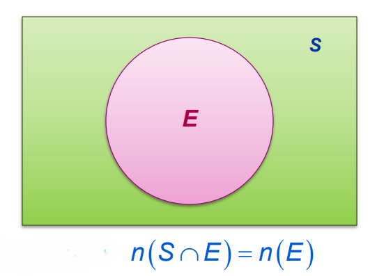
• Common points of S and E      
• An Event E on sample space S   
• Sample space S for a random experiment
• Divide it by the total number of sample points in the sample space 

Now consider a sample space S and events A, B, and C defined within it. We can derive several key properties:

Property 1:  We have

P(S|E) = P(S∩E) /P(E) = P(E) /P(E) = 1 

Also,  P(E|E) = P(E∩E) /P(E) = P(E) /P(E) = 1 

            P(S∣E) = P(E∣E) = 1

This property states that the probability of the entire sample space S given any event E is 1, as is the probability of E given E.

Property 2: For any two events A and B in the sample space, and any event E where P(E)>0,

P(A∪B∣E) = P(A∣E) + P(B∣E) − P(A∩B∣E)

If A and B are disjoint events, this simplifies to: 

P(A∪B∣E) = P(A∣E) + P(B∣E)

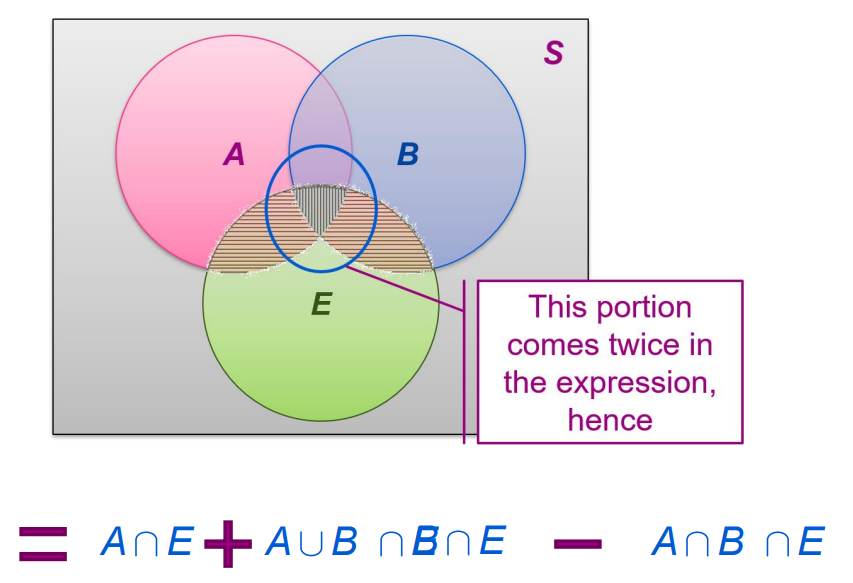
We know that

P(A∪B∣E) = P(A∪B)∩E / P(E)

Therefore, P(A∪B∣E) = P(A∩E) + P(B∩E) – P(A∩B)∩E / P(E)

                                         = P(A∩E)/P(E) + P(B∩E)/P(E) – P(A∩B)∩E / P(E)

                                         = P(A∣E) + P(B∣E) − P(A∩B∣E) 

In particular, if A and B are disjoint events, then

A∩B = ∅ ⇒ (A∩B)∩E = ∅ ⇒ P((A∩B)∩E) = 0.

Hence, P(A∪B∣E) = P(A∣E) + P(B∣E)

Property 3: 

From Property 1, we have P(S|E) = 1,

⇒ P (C∪C′)| = 1, writing S = C∪C′  

⇒ P(C|E) + P (C′ |E) = 1,        C and C’ are disjoint.

Thus,  P(C ′∣E) = 1−P(C∣E)

This property reflects the complementary nature of events, where the probability of the complement of an event C given E is 1−P(C∣E).

Let us now take an example: 

Consider the experiment of throwing two fair six-sided dice. If it is known that the sum of the number on the dice is greater than or equal to 7. What is the probability that the number on the second dice is even?

Sample space of the experiment is given by: S = {(1, 1), (1, 2), …, (1, 6), (2, 1), (2, 2), …, (2, 6), (3, 1), (3, 2), …, (3, 6), (4, 1), (4, 2), …, (4, 6), (5, 1), (5, 2), …, (5, 6), (6, 1), (6, 2), …, (6, 6)}

Let E and A are two events of this sample space defined as: E: Even number on the second dice. A: Sum is greater than or equal to 7.

Based on this definition we have, 

E = {(1, 2), (1, 4), (1, 6), (2, 2), (2, 4), (2, 6), (3, 2), (3, 4), (3, 6), (4, 2), (4, 4), (4, 6), (5, 2), (5, 4), (5, 6), (6, 2), (6, 4), (6, 6)} 

A = {(1, 6), (2, 5), (2, 6), (3, 4), (3, 5), (3, 6), (4, 3), (4, 4), (4, 5), (4, 6), (5, 2), (5, 3), (5, 4), (5, 5), (5, 6), (6, 1), (6, 2), (6, 3), (6, 4), (6, 5), (6, 6)}

The required probability is nothing but the probability of common elements of E and A, taking A as a sample space. Common elements of E and A = {(1, 6), (2, 6), (3, 4), (3, 6), (4, 4), (4, 6), (5, 2), (5, 4), (5, 6), (6, 2), (6, 4), (6, 6)}

Hence, the required probability = 12/21 {as total elements of A are 21} 

Let us calculate the same probability using the formula. We have to find the probability of event E given that event A has already occurred., we have

P(E|A) = P(E∩A)/P(A) = 1/36 x 21/36 = 12/21

Multiplication Theorem on Probability

The multiplication rule or theorem helps in finding the probability that two events A and B both occur. The rule is derived from conditional probability and is expressed as:

P(A∩B) = P(A∣B)⋅P(B) or P(A∩B) = P(B∣A)⋅P(A)

Example: Consider drawing two cards at random from a deck without replacement. The probability of drawing an ace first and a king second is calculated as follows:

P(E) = 4/52 = 1/13 (probability of an ace in the first draw)

P(F∣E) =  4/ 51 (probability of a king given the first card was an ace)

Thus: P (E ∩ F) = 1/13 x 4/51

Multiplication rule of probability for more than two events:

Suppose A, B, and C are three events defined on a sample space, then we have

P(E ∩ F ∩ G) = P(E) P(F|E) P(G|(E ∩ F)) = P(E) P(F|E) P(G|EF)

Similarly, this rule can be extended for n events.

Independent Events

Independent events are events where the outcome of an event does not affect the outcome of other events. 

For such events: P(A∩B) = P(A) × P(B)

For example, in the experiment of tossing two coins simultaneously, the toss of one coin does not affect the toss of the second coin. 

Mathematically speaking if the conditional probability of an event given that another event has already occurred is the same as the probability of the event, then the events are said to be independent. 

Formally we can define independent events as follows:

Definition: Two events A and B are said to be independent, if

P(B|A) = P(B) provided P(A) ≠ 0

P(A|B) = P(A) provided P(B) ≠ 0, 

From the above condition, we have

P(A ∩ B) = P(A) P(B) |A = P(A).P(B) or P(A ∩ B) = P(B) P(A) |B = P(B).P(A)

We can define independent events in other words as follows: 

Definition: Let A and B be two events associated with the same random experiment, then A and B are said to be independent if

P(A ∩ B) = P(B ∩ A) = P(A) . P(B) = P(B) . P(A)

Given the above definition we can define, two events are said to be dependent if

P(A ∩ B) ≠  P(A) . P(B)

Example: Suppose an urn contains 3 white balls and 7 red balls. Suppose 2 balls are chosen at random with replacement. What is the probability of getting red balls in each draw? Let A be the event that the first ball drawn is red and B be the event that the second ball drawn is red.

P(A) = P(the first ball is red ball) = 3/10.

Now, we know that the first ball drawn is red, then 

P(the second ball is red given the first ball was red) 

P(B) = P(B | A) = 3/10. 

Hence, P(AB) = P(A) x P(B) = (3/10) x (3/10) = 9/100 = 0.09.

Bayes’ Theorem

Sometimes we are interested in knowing the reverse probabilities, i.e., when an event has already occurred, and we want to determine the cause behind it. Bayes’ theorem helps in finding such probabilities. Before diving into Bayes’ theorem, let’s first go through some basic definitions.

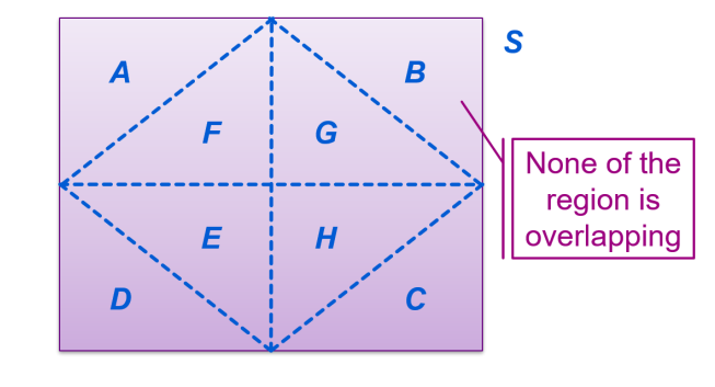
Area(S) = sum of areas of regions A, B, C, D, E, F, G and H

S is the sample space. 

A, B, C, D, E, F, G, and H are partitions of S

Partition of a Sample Space

A set of events E 1, E2,…, En represents a partition of a sample space S if:

• The events Eᵢ are mutually exclusive, i.e., Eᵢ ∩ Eⱼ = ∅ for i ≠ j.
• The events are exhaustive, meaning E₁∪E₂∪…∪Eₙ = S.
• Each event Eᵢ has a non-zero probability, P(Eᵢ)>0 for all i = 1,2,…,n.

Theorem of Total Probability

Let {E₁, E₂,…, En} be a partition of the sample space S, and let A be any event associated with S. Then, the probability of A is given by:

P(A)=P(E₁)P(A∣E₁)+P(E₂)P(A∣E₂)+…+P(Eₙ)P(A∣Eₙ)

Proof: From the figure, we have

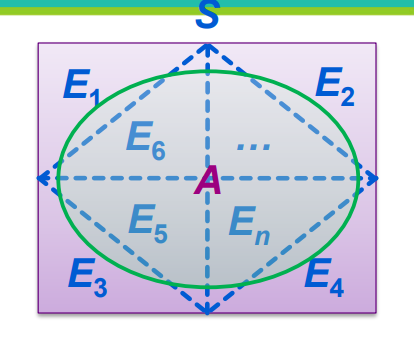
S = E₁ ∪ E₂ ∪……..∪ Eₙ and Eᵢ ∩ Eⱼ = ∅ for i ≠ j,  i,j = 1,2…n

and  P(Eᵢ)>0 for all  i – 1,2,…,n

For any event A of S = A ∩ S

                                       =  A ∩ E₁ ∪ E₂ ∪……..∪ Eₙ

                                       = A ∩ E₁ ∪ A ∩ E₂ ∪……..∪ A ∩Eₙ (Distributive property of intersection over the union of sets )

Now A ∩ Eᵢ ⊂ Eᵢ  and A ∩ Eⱼ ⊂ Eⱼ

Therefore Eᵢ∩Eⱼ = ∅ for i ≠ j,  i,j = 1,2…n

Thus P(A) = P[A ∩ E₁ ∪ A ∩ E₂ ∪……..∪ A ∩Eₙ]

                     = P(A ∩ E₁) ∪ P(A ∩ E₂) ∪……..∪ P(A ∩Eₙ)

By multiplication rule of probability, we have

P(A ∩ Eᵢ) = P(Eᵢ) P(A|Eᵢ) 

Therefore, P(Eᵢ) ≠ 0 ∀ i = 1,2,….n

(P(A)=P(E₁)P(A∣E₁)+P(E₂)P(A∣E₂)+…+P(Eₙ)P(A∣Eₙ)

i = 1n = P(Eᵢ)P(A∣Eᵢ)

Example: 

Suppose Box I contains 9 red and 7 white balls. Box II contains 5 red, 8 white, and 6 blue balls. Box III contains 7 red, 10 white, and 4 blue balls. The probabilities of choosing Box I, Box II, and Box III are 3/8, 2/5, and 9/40 respectively. A box is chosen, and then a ball is drawn. Find the probability of drawing a white ball.

Let B₁ be the event of choosing Box I, B₂ the event of choosing Box II, and B₃ the event of choosing Box III. Let W be the event of drawing a white ball. By the theorem of total probability:

P(W) = P(B₁)P(W∣B₁)+P(B₂)P(W∣B₂)+P(B₃)P(W∣B₃)

Substituting the values:

P(W) = (3/8 × 7/16)+( 2/5 × 8/19)+( 9/40 × 10/21)

P(W) = 21/128 + 16/95 + 3/28

            = 0.1641 + 0.1684 + 0.1071 = 0.4396

           ≈ 0.4396

Bayes’ Theorem: If E₁, E₂, …, Eₙ are n nonempty events that constitute a partition of sample space S and A is any event of nonzero probability, then

P (Eᵢ|A) = P(Eᵢ) P (A|Eᵢ) / J=1nP(Eⱼ) P (A|Eⱼ) for any i = 1,2,3…n

Proof: By the definition of conditional probability, we know that

P(Ei∣A) = P(E₁)P(A∣E₁)+P(E₂)P(A∣E₂)+…+P(Eₙ)P(A∣Eₙ)

P (Eᵢ|A) = P(Eᵢ) P (A|Eᵢ) / J=1nP(Eⱼ) P (A|Eⱼ) for any i = 1,2,3…n

The events E₁, E₂, …, Eₙ are called hypotheses. The probability P(Eᵢ) is called the prior probability of the hypothesis Eᵢ. The conditional probability P(Eᵢ|A) is called the posterior probability of the hypothesis Eᵢ.

​Example:

Consider the previous example. Now, calculate the probability that Box III was chosen given that a white ball was drawn. By Bayes’ theorem:

P(B₃∣W) = P(B₃) P(W|B₃) / P(B₁) P(W|B₁) + P(B₂) P(W|B₂) +P(B₃) P(W|B₃) 

                  = 0.1071 / 0.1641 + 0.1684 + 0.1071 = 0.1071 /0.4396 = 0.2436 

Random Variables

A random variable is a function that assigns a unique real number to each outcome of a random experiment. For example, consider tossing a coin four times. The sample space S is:

S={HHHH,HHHT,HHTH,HHTT,HTHH,HTHT,HTTH,HTTT,THHH,THHT,THTH,THTT,TTHH,TTHT,TTTH,TTTT}

Let X denote the number of heads obtained. X takes values 0, 1, 2, 3, or 4. The probability distribution of X is:

P(X = 0) = 1/16, P(X = 1) = 4/16, P(X = 2) = 6/16, P(X = 3) = 4/16, P(X = 4) = 1/16

Probability Distribution of a Random Variable

Consider our previous experiment of tossing a coin 4 times. 

X = number of heads obtained in 4 tosses. 

X can take any value from 0, 1, 2, 3 and 4. 

Now, observe that X will take the value 0 when all four tosses end in the tail, i.e., the outcome (TTTT). Similarly, X will take the value 1 when one of the tosses results in head, i.e., the outcomes (HTTT), (THTT), (TTHT) and (TTTH), and so on. 

Each outcome of the experiment has an equal probability of occurrence 

Thus the probability that X can take the value 0 is 1/16. 

We write it as P(X = 0) = 1/16. 

Similarly, the probability of any one of the outcomes (HTTT), (THTT), (TTHT) or (TTTH) is P((HTTT) or (THTT) or (TTHT) or (TTTH)) = 4/16 = 1/4. 

Thus, the probability that X can take value 1 is 1/4.

 We write P(X = 1) = 4/16 = ¼

Similarly, P({(HHTT), (HTHT), (HTTH), (THHT), (THTH), (TTHH)} = P(X = 2) = 6/16 = 3/8, 

P({(HHHT), (HHTH), (HTHH), (THHH)} = P(X = 3) = 4/16 = 1/4, 

P({(HHHH)} = P(X = 4) = 1/16. 

Such kind of description of values of random variables along with the corresponding probabilities is called the probability distribution of the random variable X. 

Generally, we can define the probability distribution of X as follows: Definition: The probability distribution of a random variable X is the system of numbers.

X : x₁ x₂… xₙ

P(X) : p₁ p₂ … pₙ 

Where pᵢ > 0, i =1npᵢ = 1, i = 1,2….n

The real numbers x₁, x₂, …, xₙ are the possible values of the random variable X, and pᵢ (i = 1, 2, …, n) is the probability of random variable X taking the value xᵢ, i.e., P(X = xᵢ) = pᵢ.

Example: 

Let us now consider an experiment of drawing three cards from a pack of 52 playing cards. Let us now find the probability distribution of the number of aces. 

Suppose X is the random variable indicating the number of aces. Let’s find the probability distribution of X. 

Observe that X can take values 0, 1, 2, or 3 as there are 4 aces in a pack of 52 playing cards. 

Now, P(X = 0) = Probability of getting no ace = Probability of choosing 3 other cards = C(48, 3)/C(52, 3) = 4324/5525 

The corresponding probabilities are given by: 

P(X = 1) = Probability of getting one ace and two other cards = {C(4, 1) x C(48, 2)}/ C(52, 3) = 1128/5525 

P(X = 2) = Probability of getting 2 aces and one other card = {C(4, 2) x C(48, 1)}/C(52, 3) = 72/5525 

P(X = 3) = probability of getting 3 aces = C(4, 3)/C(52, 3) = 1/5525. 

Note that all the probabilities are positive and between 0 and 1. 4324 

Observe that P(X) = 4324/5525 + 1128 / 5525 + 72 /5525 + 1/5525 = 1

Hence, the probability distribution of the number of aces is given by: 

X	0	1	2	3
P(X)	4324/5525	1128 / 5525	72 /5525	1/5525

Let us now consider the following probabilities of a random variable X. Determine whether it is a probability distribution of X:

X	0	1	2
P(X)	0.4	0.4	0.2

Note that all the probabilities are between 0 and 1. The only thing that remains to show is that the probabilities sum up to 1. 

Hence, 0.4 + 0.4 + 0.2 = 1 As the probabilities add up to 1. The given description defines a valid probability distribution for X.

Now let us find the probability P(X > 0)

P(X > 0) = P(All the values greater than 0 (exclusive) 

                  = P(X = 1) + P(X = 2) = 0.4 + 0.2 = 0.6

The mean of a Random Variable

The mean or expectation of a random variable X is the weighted average of its possible values, with weights being the probabilities of those values:

E(X)= i xᵢ P(X = xᵢ)

Definition: Let be a random variable whose possible values x₁,x₂,….xₙ, occur with probabilities p₁,p₂, pₙ respectively. 

The variance is given by

i =1nxᵢ pᵢ. It is denoted by

For the example of tossing a coin four times, the mean of X is calculated as:

E(X) = 0 × 1/16 + 1× 4/16 + 2× 6/16 + 3 × 4/16 + 4 × 1/16 = 2

The mean describes the central tendency of the distribution.

Variance of a Random Variable

Mean is representative of a probability distribution which describes the location of the random variable. Sometimes it is not sufficient to describe the location parameter. We also need to describe the variability of the random variable. 

Variance is one such parameter that describes the variability or dispersion of the distribution. 

Sometimes random variables with different probability distributions can have equal means and in that case, variance plays an important role in describing the behavior of the random variables.

Definition: Let be a random variable whose possible values x₁,x₂,….xₙ, occur with probabilities p₁,p₂, pₙ respectively. 

The variance of is given by

i =1nxᵢ – ² pᵢ or equivalently E (x-²)

It is denoted by ²ₓ. Where E(x) – is the mean of X.

The non-negative number

                        ₓ  = √Var X = √i =1nxᵢ – pᵢ 

is called the standard deviation of the random variable X. Alternatively, the variance of the random variable X is also given by:

           Var X = ²ₓ = EX² – [EX]² where EX² = i =1nxᵢ² ² pᵢ

Example: Let us now consider the experiment of tossing a coin 4 times. The probability distribution of the random variable X which denotes the number of heads is given by: 

X = xᵢ	0	1	2	3	4
P(X) = xᵢ	1/16	1/4	3/8	1/4	1/16

Now, the mean of X is 2 as we calculated before. Now, the variance of the random variable is given by: 

                               Var X = EX² – [EX]² 

For this, let us calculate the expectation E(X²) first. 

EX²  = i =1nxᵢ² pᵢ = 1/16 + 0 x 1² +1 x 4² + 2 x 6² + 3 x 4² + 4 x 1²

                       = 1/16 + 16 + 72 + 48 + 4

                        = 1/16 x 140 = 8.75     

Hence, the variance is given by: 

Var(X) = E(X²) – [E(X)]² = (8.75) – (2)² = 4.75 

Let’s Conclude

In conclusion, Probability is a fundamental chapter in CBSE Class 12 Mathematics that equips students with the tools to analyze random events and make informed predictions about uncertain outcomes. Throughout this Probability chapter, we’ve explored essential concepts such as conditional probability, independence, and the application of various probability distributions, all of which are crucial for deeper studies in fields like statistics, economics, and data science. By mastering the principles outlined in the Probability chapter, students can enhance their analytical skills and apply mathematical reasoning to real-life scenarios effectively.

With the comprehensive resources provided by iPrep, including engaging animated videos and practical exercises, you are well-equipped to conquer the complexities of Probability. Remember, the key to excelling in this chapter lies in understanding the concepts and practicing them regularly. Embrace the challenge, and let the journey into the world of Probability open doors to new academic and professional opportunities!