Linear Programming – Complete Guide For Class 12 Math Chapter 12

Welcome to iPrep, your Learning Super App. Our learning resources for the chapter, Linear Programming in Mathematics for Class 12th are designed to ensure you grasp this concept with clarity and perfection. Whether you’re studying for an upcoming exam or strengthening your concepts, our engaging animated videos, practice questions and notes offer you the best of integrated learning with interesting explanations and examples. 

The chapter “Linear Programming” in Class 12th Math introduces students to the method of optimizing a linear objective function, subject to a set of linear inequalities or constraints. This chapter covers the formulation of linear programming problems, graphical methods for solving problems in two variables, and the concept of feasible and optimal solutions. Linear Programming is essential for various fields such as economics, operations research, and management, where it helps in making decisions about resource allocation, production scheduling, and cost minimization. Understanding this chapter is crucial for students pursuing higher studies in mathematics, economics, and business.

Linear Programming

Imagine two apparel factories supplying goods to three different stores, each with its specific daily demand. The challenge? Minimizing the transportation costs while fulfilling these demands. This scenario perfectly exemplifies a Linear Programming Problem (LPP), where the goal is to optimize a particular outcome—in this case, cost—within certain constraints.

Learning Linear Programming with An Example

Let’s delve into the concepts of Linear Programming through this real-world example.

The Scenario: Apparel Design Factories and Stores

Factory A:

• Maximum Capacity: 2200 Apparel/Day
• Transportation Costs:

              Store P: Rs 2/Apparel

              Store Q: Rs 1.5/Apparel

              Store R: Rs 2.2/Apparel

Factory B:

• Maximum Capacity: 2800 Apparel/Day
• Transportation Costs:

              Store P: Rs 1/Apparel

              Store Q: Rs 2.5/Apparel

              Store R: Rs 1.5/Apparel

Stores:

• Store P: Daily Demand = 1500 Apparel
• Store Q: Daily Demand = 1800 Apparels
• Store R: Daily Demand = 1700 Apparels

The Problem

The factories need to meet the daily requirements of all three stores at the minimum transportation cost. This type of problem is an “Optimization Problem,” where we aim to find the best possible solution among several alternatives under specific constraints.

What is an Optimization Problem?

An Optimization Problem seeks to maximize or minimize a particular outcome—such as profit or cost—among existing alternatives. Some key characteristics include:

• Multiple alternatives to choose from.
• Accompanied by certain constraints.
• The aim is to identify the optimal solution.

A special class of these problems is known as Linear Programming Problems (LPP), which we will now explore in more detail.

Understanding Linear Programming Problems

Linear Programming Problems (LPP) are widely applicable in various fields, including industry, commerce, and management science. Let’s see how our apparel design scenario fits into the framework of an LPP.

Mathematical Formulation of the LPP

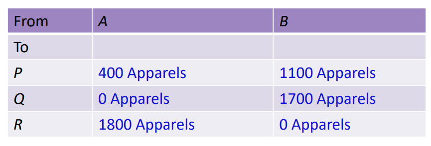
To minimize transportation costs, we need to determine how much apparel should be sent from factories A and B to stores P, Q, and R.

Let: 

• x = Units sent from Factory A to Store P
• y = Units sent from Factory A to Store Q
• 2200−x−y = Units sent from Factory A to Store R

x ≥ 0, y ≥ 0  and 2200 – x – y ≥ 0 or  x ≥ 0, y ≥ 0 and x + y ≤ 2200

Similarly, from Factory B:

• 1500−x = Units sent to Store P
• 1700−y = Units sent to Store Q
• 2800−(1500−x+1700−y) = Units sent to Store R

1500 – x ≥ 0, 1700 –  y ≥ 0  and x + y – 400 ≥ 0 or x ≤ 1500, y ≤ 1700 and x + y ≥ 400

The objective is to minimize the transportation cost Z, given by: Z = 2x + 1.5y + 2.2 (2200 − x − y) + 1(1500 − x) + 2.5 (1700 − y) + 1.5 (x + y − 400) 

Simplifying, we get: Z = 0.2x − 1.7y + 9990

The Complete Mathematical Formulation

The entire problem can be summarized mathematically as:

• Objective Function: Minimize Z = 0.2x − 1.7y + 9990
• Subject to Constraints:  

1. x + y ≤ 2200
2. x + y ≥ 400
3. x ≤ 1500
4. y ≤ 1700
5. x ≥ 0, y ≥ 0

Key Concepts in Linear Programming Problem

There are various key concepts in linear programming. These include-

Objective Function: A linear function in several variables that need to be minimized or maximized. In our case, it represents the total transportation cost.

In our “Apparel Design” example the objective function is: Z = 0.2x − 1.7y + 9990

Which represents the total cost of transportation of apparel from factories A and B to stores at P, Q, and R.

Decision Variables: The variables x and y upon which the objective function depends.

In our “Apparel Design” example the decision variables are ‘x’ and ‘y’ which represent the total units to be transferred from factory A to stores at P and Q.

Constraints: The linear inequalities or restrictions on the variables, such as production capacities and store demands.

In our “Apparel Design” example the conditions x ≥ 0, and y ≥ 0 are non-negativity constraints.

General Form of a Linear Programming Problem

In general, a Linear Programming Problem is represented as:

• Maximize (or Minimize) Z = c₁x₁+ c₂x₂ +⋯+ cₙxₙ
• ​Subject to Constraints: a₁₁x₁+a₁₂x₂+⋯+a₁ₙxₙ ≤ b₁

          𝑎₂₁𝑥₁+𝑎₂₂𝑥₂+⋯+𝑎₂ₙ𝑥ₙ ≤ 𝑏₂

                           ……

               𝑥₁ ≥ 0,𝑥₂ ≥ 0,…,𝑥ₙ ≥ 0

Where, Z is the objective function, x₁, x₂ , …, xₙ are decision variables and c₁, c₂ , …, cₙ , a₁₁, a₁₂, …a₁ₙ, b₁ , b₂ , …bₙ are constants

The solution to Linear Programming Problems

A solution to an LPP satisfies all constraints. 

Feasible Solution: A Feasible Solution satisfies both the constraints and non-negativity conditions. 

The Feasible Region is the set of all feasible solutions, while the Infeasible Region contains points that do not satisfy all constraints.

The Optimal Feasible Solution is the point within the feasible region that gives the optimal value (maximum or minimum) for the objective function.

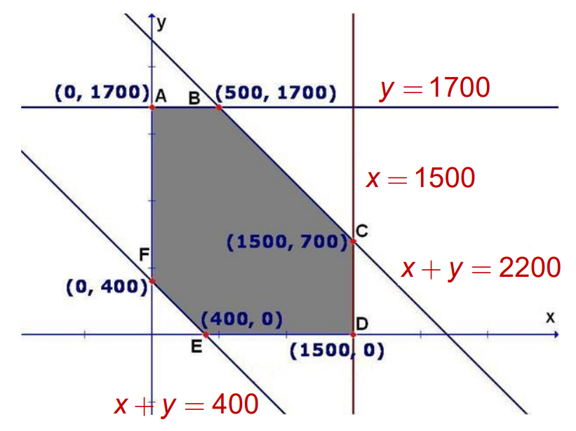
For our “Apparel Design” example the feasible region (shaded region) is shown in the figure with some feasible solutions to the problem.

Related Terms to Linear Programming 

• As we can see within the feasible region, there can be infinitely many points that satisfy all the constraints. Then the question arises how do we select the optimal solution of an LPP? 
•  To answer this question we have some theorems which determine that a particular feasible solution is optimal too for a given LPP.

Theorem 1:

Statement: Let R be the feasible region (convex polygon) for an LPP and let Z = ax + by be the objective function. When Z has an optimal value (maximum or minimum), where the variables x and y are subject to constraints described by linear inequalities, this optimal value must occur at a corner point (vertex) of the feasible region.

 In our example, the feasible region is represented by the convex polygon ABCDEF. Hence according to the above theorem optimal solution of our LPP must lie on one of the vertex of the polygon ABCDEF.

Theorem 2: 

Statement: Let R be the feasible region for an LPP, and let Z = ax + by be the objective function. If R is bounded, then the objective function Z has both a maximum and a minimum value on R, and each of these occurs at a corner point (vertex) of R. 

In our example, the feasible region is a bounded region represented by a convex polygon ABCDEF. Hence according to the above theorem objective function i.e. Z = 0.2x – 1.7y + 9990 has its maximum and minimum value on ABCDEF and each of these occurs at one of the vertex of the polygon ABCDEF.

Graphical Method to Solve a Linear Programming Problem

For LPPs with two decision variables, graphical methods can be employed. One such method is the Corner Point Method:

• Graph the inequalities of the LPP in the coordinate system.
• Identify the feasible region.
• Determine the corner points (vertices) of the feasible region.
• Evaluate the objective function Z=ax+by at each corner point.
• The maximum and minimum values of Z give the optimal solution.

Example: Solving the Apparel Design Problem

To minimize the transportation cost Z = 0.2x − 1.7y + 9990 subject to the constraints, we:

Solution: We’ll first sketch the feasible region of the given LPP. Then we’ll find the value of the objective function at each corner point of the feasible region.

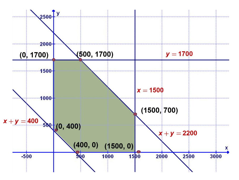
Now calculate the value of the objective function at each corner point: 

• At point (400, 0), Z = 0.2(400) – 1.7(0) + 9990 = 10070
• At point (1500, 0), Z = 0.2(1500) – 1.7(0) + 9990 = 10290 
• At point (1500, 700), Z = 0.2(1500) – 1.7(700) + 9990 =11480 
• At point (1500, 1700), Z = 0.2(1500) – 1.7(1700) + 9990 = 13180 
• At point (0, 1700), Z = 0.2(0) – 1.7(1700) + 9990 = 12880 
• At point (0, 400), Z = 0.2(0) – 1.7(400) + 9990 = 10670.

The minimum occurs at point (400, 0) and the minimum cost of transportation is 10070. 

Corner Point Method

• When a feasible region is unbounded Let M and m be the largest and smallest value of objective function Z = ax + by respectively and these values occur at points (x₁, y₁) and (x₂, y₂) respectively. 
• Now, M will be the maximum value of Z, if the open half plane determined by ax + by > M has no point in common with the feasible region other than (x₁, y₁). Otherwise, Z has no maximum value. 
• Similarly, m is the minimum value of Z, if the open half plane determined by ax + by < m has no point in common with the feasible region other than (x₂, y₂). Otherwise, Z has no minimum value.

Example: 

Solve the following LPP graphically:

Minimise Z = 3x + 5y 

Subject to x + 3y ≥ 3, x + y ≥ 2, and x, y ≥ 0

Solution: We’ll first sketch the feasible region of the given LPP. Then we’ll find the value of the objective function at each corner point of the feasible region. 

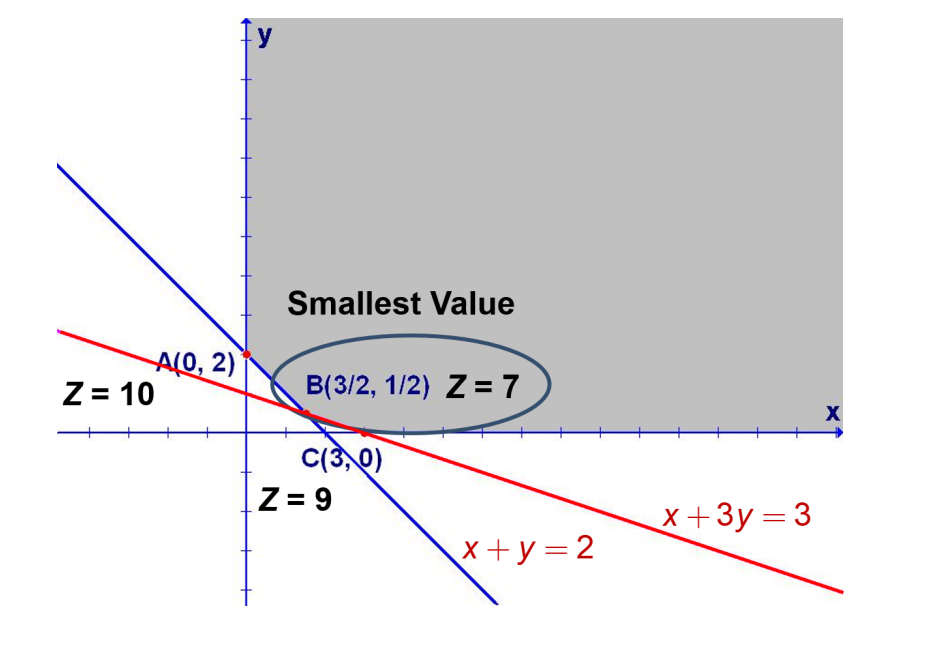
Now we’ll check whether the open half plane determined by 3x + 5y < 7 and feasible region have common points other than B(3/2, 1/2). 

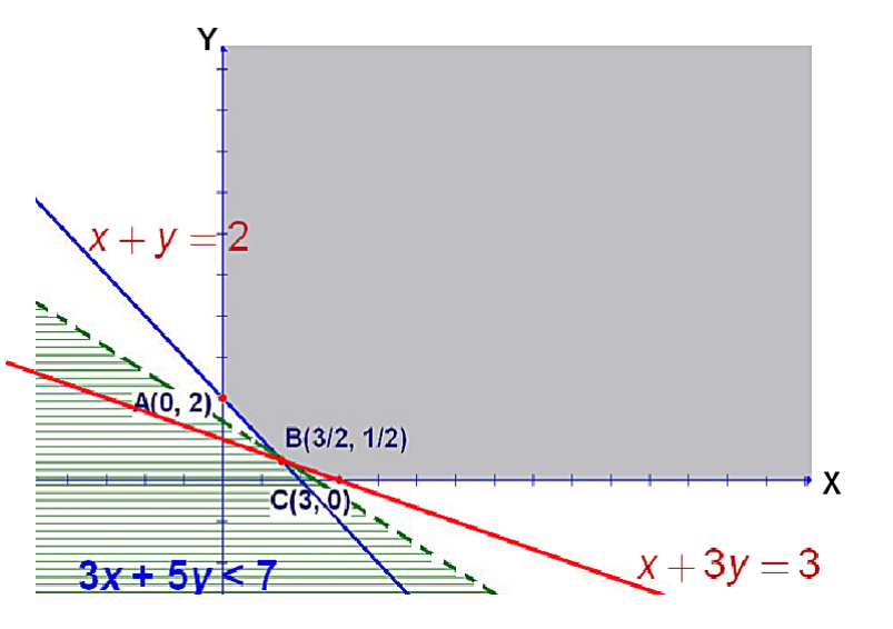
Feasible region and open half plane 3x + 5y < 7 have only one point in common which is B(3/2, 1/2). Hence 7 is the minimum value of the objective function which occurs at point B(3/2, 1/2).

Let’s Conclude

In conclusion, the chapter “Linear Programming” from CBSE Class 12 Math plays a crucial role in developing problem-solving and decision-making skills. It teaches students how to optimize outcomes under given constraints, whether it’s minimizing costs or maximizing profits. With practical applications across various industries, mastering Linear Programming is highly beneficial for future endeavors in fields like economics, operations research, and management. By leveraging the engaging resources available on iPrep, such as animated videos, practice questions, and detailed notes, students can fully grasp the concepts and excel in the chapter “Linear Programming” for Class 12 Math. Remember, understanding the fundamentals of Linear Programming is key to excelling not only in exams but also in real-world decision-making scenarios.