Complete Guide For Class 9 Math Chapter 12 – Statistics

Our learning resources for Mathematics Class 9 ‘Statistics’ chapter 12 are designed to ensure that you grasp this concept with clarity and perfection. Whether you’re studying for an upcoming exam or strengthening your concepts, our engaging animated videos, practice questions, and notes offer you the best of integrated learning with interesting explanations and examples.

Our comprehensive approach ensures that you have access to everything you need to have an in-depth understanding of the chapter Statistics. From detailed notes to interactive exercises, our materials are tailored to meet your learning needs and help you excel in your studies. Get ready to dive into an enriching educational experience that will make mastering this chapter a breeze.

Statistics is the art of collecting, organizing, analyzing, interpreting, and presenting data. This chapter introduces you to basic statistical concepts. Learn about raw data, frequency distribution tables, grouped data, and measures of central tendency like mean, median, and mode. Understand how to handle large datasets and draw meaningful conclusions from them.

Welcome to another insightful exploration of Class 9 Mathematics! In this blog, we will dive into Chapter 12 – Statistics. This chapter provides a comprehensive understanding of the fundamentals of statistics, its definition, types of data, and various methods of data presentation and analysis. Let’s get started!

Introduction to Statistics

Definition of Statistics

Statistics is a branch of mathematics that deals with the collection, presentation, analysis, and interpretation of numerical data. The term “statistics” can be understood in both singular and plural senses:

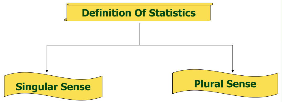
• Singular Sense: It refers to the science of collecting, presenting, analyzing, and interpreting numerical data.
• Plural Sense: It denotes numerical facts or observations collected with a specific purpose.

For example, the number of males and females in a particular city is a statistical data point.

Types of Statistical Data

Statistical data can be classified into two main categories: Primary Data and Secondary Data.

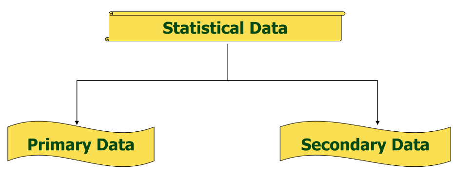
Primary Data

Primary data is the data collected firsthand by an investigator with a specific plan or design in mind. It is:

• Reliable
• Relevant
• Original

Example: Data obtained from a population census by the office of the Registrar General and Census Commissioner.

Secondary Data

Secondary data is the data that has been collected by someone else and is obtained from published or unpublished sources. It requires greater care to ensure its relevance and accuracy.

Example: Using the latest copy of ‘Educational Statistics of India’ to find the literacy rate of India.

Presentation of Data

Once data is collected, it needs to be presented in a way that highlights its key features. This process is called data presentation. For instance, consider the marks obtained by five students in a Mathematics test (out of 100):

80, 95, 72, 90, 69

In its raw form, this data can be arranged in various ways:

• Serial or Alphabetical order
• Ascending order
• Descending Order

When raw data is arranged in ascending or descending order, it is called an array or array data.

Constructing Frequency Distributions

To analyze data more effectively, it can be organized into frequency distributions. There are two types of frequency distributions: Discrete and Grouped.

Discrete Frequency Distribution

Steps to Construct:

1. Obtain the raw data.
2. Prepare a table with three columns: one for the variable (e.g., marks), one for tally marks, and one for the frequency.
3. Arrange the data in ascending order.
4. Use tally marks to record the frequency of each value.
5. Summarize the tally marks to obtain the frequency for each value.

Example: Consider the marks obtained by 27 students:

80, 95, 72, 90, 69, 80, 75, 75, 90, 85, 72, 80, 85, 75, 85, 72, 85, 98, 72, 45, 36, 80, 95, 69, 90, 56, 80

The resulting frequency distribution table will show the number of students who obtained each mark.

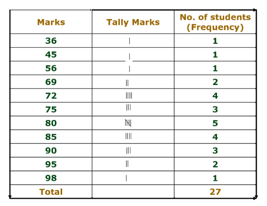
This is called an ungrouped frequency distribution or a frequency distribution table.

Grouped Frequency Distribution

When data is extensive, it can be grouped into classes or intervals. Each class has a range, known as the class interval.

Steps to Construct:

1. Determine the maximum and minimum values in the data.
2. Decide the number of classes (usually 5 to 15).
3. Calculate the class interval.
4. Assign each data point to a class and record the tally marks.
5. Summarize the tally marks to get the frequency for each class.

Example: Marks of students grouped into intervals:

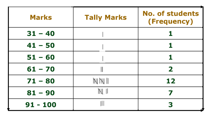
This is known as a grouped frequency distribution.

Note: This is the inclusive method.

Grouped Frequency Distribution:

Exclusive Method: When the class intervals are so fixed that the upper limit of one class is the lower limit of the next class, it is known as the exclusive method of classification.

In this method, the upper limit of a class is not included in the class.

Inclusive Method: In the inclusive method of classification, the classes are so formed that the upper limit of a class is included in that class.

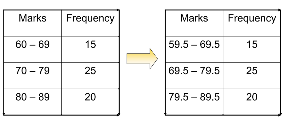
How to convert from Inclusive to Exclusive Form: 

• Find the difference between the upper limit of a class and the lower limit of its succeeding class. Denote this by h.
• Add half of this difference to each of the upper limits of the class – intervals.
• Subtract half of this difference from each of the lower limits of the class – intervals.
• So, if (a – b) is a class in an inclusive method, then in an exclusive method it becomes

 { (a – h/2) – (b + h/2) }.

Now, look at the example given below:

Points to remember:

• Classmark = Upper Limit + Lower Limit / 2
• Range = Maximum Value – Minimum value

Graphical Representation of Data

Data can also be represented graphically for better visualization. Common graphical methods include:

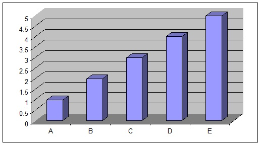
• Bar Graphs: Pictorial representation using bars of uniform width.

Algorithm:

1. Take a graph paper and draw two lines perpendicular to each other and call them horizontal and vertical axes.
2. Along the horizontal axis, mark the information given in the data like days, weeks, places, etc. at uniform gaps.
3. Choose a suitable scale to determine the heights of the rectangles or bars and then mark the heights on the vertical axis.
4. Drawbars or rectangles of equal width and height are marked in Step 3 on the horizontal axis with equal spacing between them.

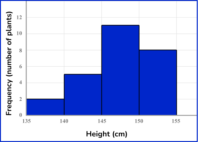
• Histograms: Graphical representation using rectangles where class intervals are the bases, and heights are proportional to frequencies.

Algorithm:

1. Take a graph paper and draw two perpendicular lines, one horizontal (representing X-axis) and one vertical (representing Y-axis), intersecting at O(say). Mark them as OX and OY.
2. Choose a suitable scale along the X-axis and represent class limits on it.
3. Choose a suitable scale for the Y-axis and mark frequencies along the Y-axis.
4. Construct rectangles with class intervals as bases and respective frequencies as heights.

NOTE: The scale for the X-axis may not be the same as the scale for Y-axis.

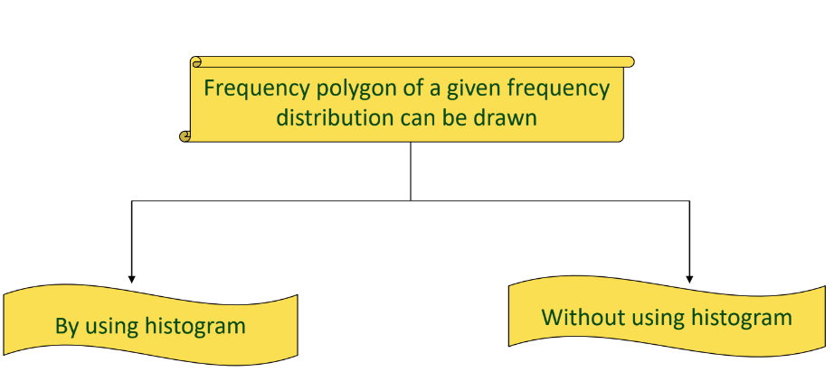
• Frequency Polygons: Line graphs connecting the midpoints of class intervals.

Measures of Central Tendency

Central tendency measures provide a single value that represents the center of a data set. The commonly used measures are:

• Arithmetic Mean (Average): Sum of all observations divided by the number of observations.
• Median: Middle value that divides the data into two equal parts.
• Mode: Most frequently occurring value.

Arithmetic Mean: The mean or average of several observations is the sum of values of the values of all the observations divided by the total number of observations.

Example: Arithmetic Mean

If five people spend the following hours in social work: 10, 7, 13, 20, 15, the mean is calculated as:

Mean = 10+7+13+20+15/5 =13

Median: The median of a distribution is the value of the variable that divides the distribution into two equal parts i.e. it is the value of the variable such that the number of observations above it is equal to the number of observations below it.

Algorithm

1. Arrange the observations(values of the variate) in ascending or descending order of magnitude.
2. Determine the total number of observations, say, n.
3. If n is, then Median = Value of (n + 1)/2 th observation.
4. If n is , then Median = {Value of (n/2)th observation + Value of (n + 1)/2 th observation}/2.

Example: Median

For the data: 25, 34, 31, 23, 22, 26, 35, 28, 20, 32, the median is:

1. Arrange the data: 20, 22, 23, 25, 26, 28, 31, 32, 34, 35.
2. Since n = 10, the median is the average of the 5th and 6th values:

Median = 26+28/2 = 27

Mode: Mode is the value that occurs most frequently in a set of observations and around which the other items of the set cluster densely. Thus, the mode of a frequency distribution is the value of the variable which has a maximum frequency.

Example: Mode 

Find the mode of the following data: 110, 120, 130, 120, 110, 140, 130, 120, 140, 120.

Since the value 120 occurs a maximum number of times i.e. 4. Hence, the modal value is 4.

Note: In a moderately symmetric distribution mean, median, and mode are connected by the following formula :

Mode = 3 Median – 2 Mean

Understanding statistics is crucial for analyzing and interpreting data effectively. By mastering the concepts of data collection, presentation, and central tendency measures, students can make informed decisions based on statistical data. Keep practicing these concepts to enhance your statistical skills!

In this blog, we explored the intricacies of Class 9 Math Chapter 12 – Statistics. This chapter is essential for developing a solid foundation in the principles of statistics, including data collection, presentation, and analysis. We covered the different types of data, methods of organizing data through frequency distributions, and various graphical representations like bar graphs and histograms. Additionally, we delved into measures of central tendency such as mean, median, and mode, which are fundamental for interpreting data accurately.

Mastering Chapter 12 – Statistics equips you with valuable skills for handling and analyzing data effectively. Whether you’re preparing for exams or aiming to strengthen your understanding, our comprehensive resources are here to guide you through every step. Embrace the study materials and practice exercises to excel in Statistics and enhance your overall mathematical proficiency. Remember, the more you practice, the more proficient you’ll become in applying statistical methods to real-world scenarios. Keep exploring and refining your skills in Chapter 12 – Statistics, and you’ll find yourself well-prepared for any data analysis challenge that comes your way!