Complete Guide For Class 10 Math Chapter 13 – Statistics

Welcome to iPrep, your Learning Super App. Our learning resources for the chapter, Statistics in Mathematics for Class 10th are designed to ensure that you grasp this concept with clarity and perfection. Whether you’re studying for an upcoming exam or strengthening your concepts, our engaging animated videos, practice questions and notes offer you the best of integrated learning with interesting explanations and examples. 

The chapter Statistics introduces students to the collection, presentation, analysis, and interpretation of data. It covers key concepts such as mean, median, and mode, which are measures of central tendency used to summarize data. Students also learn about the cumulative frequency, cumulative frequency distribution, and the graphical representation of data through histograms and ogives. Additionally, the chapter delves into the calculation of the mean using different methods, including the direct, assumed mean, and step deviation methods. Understanding these statistical tools enables students to effectively analyze data, draw meaningful conclusions, and apply statistical reasoning to real-world situations.

Statistics

Statistics is a branch of mathematics dealing with data collection, organization, analysis, interpretation, and presentation. 

Let’s understand this with an Example: 

A Classroom Activity: Understanding Mean, Median, and Mode

Scenario: The teacher enters the class with six bags filled with marbles and asks the students to count the marbles in each bag.

Group Activity: The class is divided into six groups, and each group is given a bag of marbles to count.

The groups count and record the number of marbles as follows:

• Step 1: The teacher asks the students to find the total number of marbles across all groups: 25 + 20 + 20 + 16 + 21 + 18 = 120
• Step 2: Next, the students are asked to calculate the average number of marbles by dividing the total number by the number of groups:

                  Mean = 120 /6 = 20

           The mean represents the average number of marbles per group.

• Step 3: The students arrange the numbers in ascending order: 16,18,20,20,21,25

            The middle-most number is identified to calculate the median:

                  Median = 20 + 20 /2 = 20

              The median represents the middle value in the dataset.

• Step 4: Finally, the teacher asks the students to identify the number that appears most frequently:

             The model is found to be 20, as it occurs twice in the dataset.

             The mean, median, and mode are collectively known as measures of central tendency.

Central Tendency in Grouped Data

As stated in the chapter Statistics, when dealing with small, ungrouped data, we can directly apply the formulas for mean, median, and mode. However, in real-world situations, we often work with large, grouped datasets, requiring modified formulas to calculate these measures.

Mean of Grouped Data

As per the chapter statistics, for grouped data, where data is categorized into classes, the mean is calculated using the formula:

Mean = ∑𝑓ᵢ𝑥ᵢ / ∑𝑓ᵢ

• Where: 𝑥ᵢ are the class marks (midpoints of the classes).
• 𝑓ᵢ are the frequencies of each class.

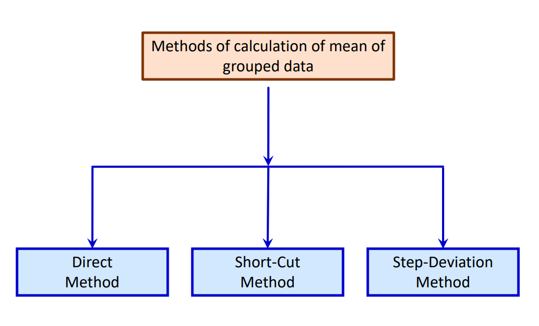
There are three methods to calculate the mean of grouped data:

• Direct Method: Class marks 𝑥ᵢ are multiplied by their corresponding frequencies 𝑓ᵢ, summed, and then divided by the total frequency.

Classmark = Upper limit of a class + Lower limit of a class / 2

Let’s understand

Suppose we have some grouped data which is being divided into n (say) classes.

Let x₁, x₂, x₃, …, xₙ are the class marks of each class. Frequencies of these classes are given by f₁, f₂, f₃, …, fₙ. Then mean of grouped data is given by: 

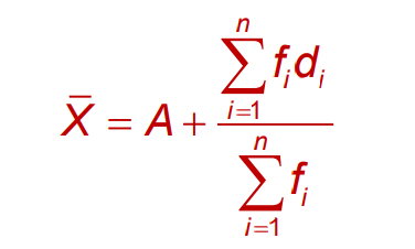
• Short-Cut Method: This method involves calculating deviations from an assumed mean, simplifying the calculation process, especially when the data is widely spread out.

Let x₁, x₂, x₃, …, xₙ are class marks of a grouped data which is being divided into n classes. Frequencies of these classes are given by f₁, f₂, f₃, …, fₙ. 

Now, taking deviations d₁, d₂, d₃, …, dₙ of these observations about some arbitrarily chosen point A (say). 

Then mean of the data is given by: 

The number A is called the assumed mean. Generally, we choose a middle value among observations to keep the deviations small.

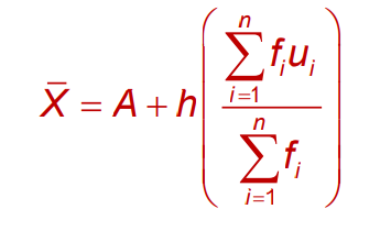
• Step-Deviation Method: This method is similar to the Short-Cut Method but further simplifies calculations by dividing deviations by a common factor, ℎ.

Let x₁, x₂, x₃, …, xₙ are class marks of a grouped data which is being divided into n classes. Frequencies of these classes are given by f₁, f₂, f₃, …, fₙ. 

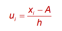
Now, taking deviations d₁, d₂, d₃, …, dₙ of these observations about some arbitrarily chosen point A (say). Deviations so found might have some factor common between them h(say). If so, then the mean of the data is given by:

Where ui is given by: 

Example:

The table below gives the percentage distribution of female teachers in the primary schools of rural areas of various states and union territories (U.T.) of India. Find the mean percentage of female teachers by all the three methods discussed in this section.

Solution: Here we take a = 50, h = 10, then dᵢ = xᵢ – 50 and uᵢ = xᵢ – 50/10

From the table above, we obtain Σfᵢ = 35, Σfᵢxᵢ = 1390,

Σfᵢdᵢ = – 360, Σfᵢuᵢ = –36.

Using the direct method, x =  Σfᵢxᵢ /Σfᵢ =  1390/35 =  39.71

Using the assumed mean method,

x =  a + Σfᵢdᵢ/Σfᵢ =  50+ (-360)/35= 39.71

Using the step-deviation method, x = a + (Σfᵢuᵢ) /Σfᵢ x h = 50+ (-36/35) x 10 = 39.71

Therefore, the mean percentage of female teachers in the primary schools of rural areas is 39.71.

Median of Grouped Data

Recall, If x₁, x₂, x₃, …, xn are some observations in ascending or descending order, then the median of these observations is given by:

Key Points: 

• For grouped frequency distribution, we first find out the cumulative frequency of all classes and also find the value of n/2.
• Now, we identify the class whose cumulative frequency is greater than (and nearest to) n/2, we call this as median class.
• After finding the median class of grouped data we use the following formula for calculating median.

                                   Median = 𝑙 + ( 𝑛/2 − 𝑐𝑓 /𝑓) × ℎ

      Where: 

• 𝑙 is the lower limit of the median class. 
• 𝑛 is the total number of observations.
• 𝑐𝑓 is the cumulative frequency of the class preceding the median class.
• 𝑓 is the frequency of the median class.
• ℎ is the class size.

Mode of Grouped Data

Key Points:

• Mode is the value that occurs most frequently in a set of observations and around which other items of the set cluster densely.
• Thus, the mode of a frequency distribution is the value of a variable that has a maximum frequency.
• In grouped frequency distribution, finding observation with maximum frequency is not possible. We can only locate classes with maximum frequency. This class is called as modal class of the observation. Mode is a value inside the modal class.
• We can find a mode of the observations from the modal class as:

                    Mode = 𝑙 + ( 𝑓₁ − 𝑓₀ / 2𝑓₁ – 𝑓₀− 𝑓₂) × ℎ

       Where:

• 𝑙 is the lower limit of the modal class.
• ℎ is the class interval.
• 𝑓₁ is the frequency of the modal class.
• 𝑓₀ and 𝑓₂ are the frequencies of the classes before and after the modal class.

Example: Calculating Mode

Consider the following dataset representing the lifetimes (in hours) of 225 electrical components:

Step 1: Identify the modal class (the class with the highest frequency, which is 60-80 hours).

Step 2: Apply the formula: 

Mode = 60 + ( 61 − 52 / 2 x  61 − 52 − 38) × 20 

           = 60 + 20 (9/32) = 60 + 5.6 = 65.6 ≈ 66 hours

Thus, the modal lifetime of the components is approximately 66 hours.

Relationship Between Mean, Median, and Mode

In a moderately symmetrical distribution, the following relationship holds:

3 × Median = Mode + 2 × Mean

Let’s Conclude

In conclusion, Chapter 13 – Statistics for CBSE Class 10th Math is an essential part of understanding how to interpret and analyze data effectively. This chapter provides a foundational grasp of statistical concepts such as mean, median, and mode, which are crucial for summarizing and drawing insights from data sets. By exploring various methods to calculate these measures, including direct, assumed mean, and step-deviation methods, students are well-equipped to handle both simple and complex data sets. The practical applications of these concepts, as demonstrated through examples and activities, highlight the relevance of statistics in real-world scenarios.

Mastering the chapter Statistics not only prepares students for their exams but also enhances their analytical skills, making them proficient in understanding and using data in everyday situations. Whether you’re looking to solidify your knowledge or explore new statistical techniques, iPrep’s resources for Chapter 13 – Statistics are designed to support and guide you through every step of your learning journey. Embrace these statistical tools, and let them empower your ability to interpret data with confidence and clarity.